Multi-Label Genre Classification-Part II
In this part, we'll be looking at some more preprocessing and BERT model training using the Huggingface library


Table of Contents
1. Import Libraries
In this section we will load and install all the libraries that we will require in the course of this project
import json
import tarfile
import pandas as pd
import re
import string
import os
from tqdm import tqdm
from pattern.text.en import singularize
from sklearn.model_selection import train_test_split
import tensorflow as tf
from transformers import BertTokenizerFast, TFBertModel
import numpy as np
import tempfile
import sys
import subprocess
from datetime import datetime
from packaging import version
import matplotlib.pyplot as plt
import seaborn as sns

%matplotlib inline
2. Data and Labels
Load the preprocessed dataframe in order to obtain the data and its labels
PATH=<YOUR_PATH>
preprocessed_df = pd.read_csv(os.path.join(PATH, 'summary_and_labels.csv'))
data = preprocessed_df.loc[:, 'Movie_Summary'].to_numpy().reshape(-1, 1)
labels = preprocessed_df.iloc[:, 3:].to_numpy()
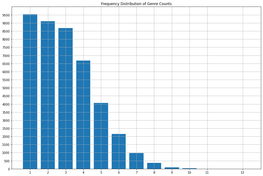
2.1 Frequency Distribution of Genre Counts
Observed the number of genres that the examples usually contain
unique, counts = np.unique(np.sum(labels, axis = 1), return_counts = True)
plt.figure(figsize = (15, 10))
plt.bar(unique, counts);
plt.xticks(unique);
plt.yticks(np.arange(0, 10000, 500))
plt.title('Frequency Distribution of Genre Counts');
plt.grid(axis = 'both')
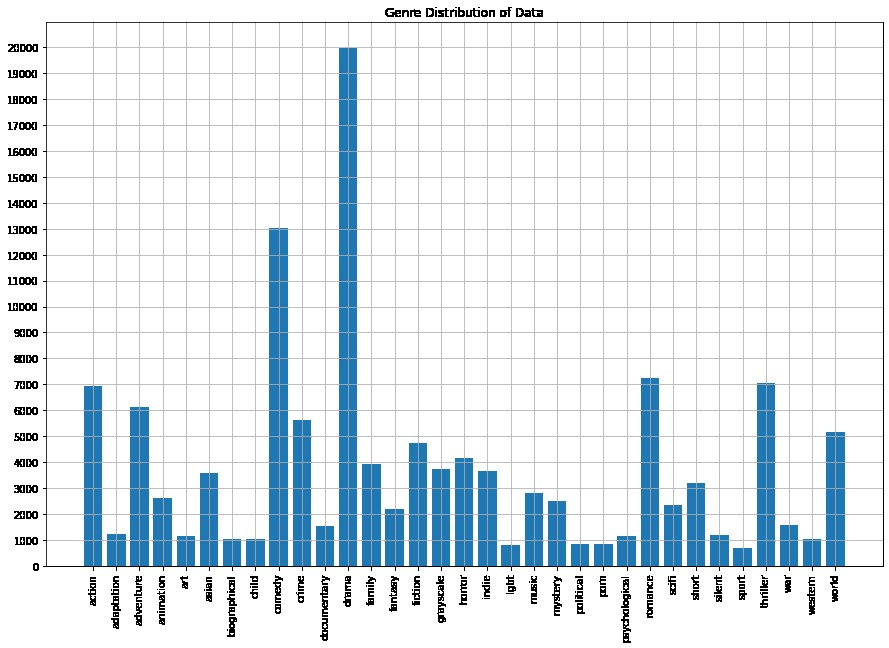
2.2 Genre Distribution of Data
Observe the genres most frequent in our dataset
plt.figure(figsize = (15, 10))
plt.bar(np.arange(1, 34, 1), np.sum(labels, axis = 0));
plt.xticks(np.arange(1,34,1), labels = preprocessed_df.iloc[:, 3:].columns, rotation = 90);
plt.yticks(np.arange(0, 21000, 1000))
plt.title('Genre Distribution of Data');
plt.grid(axis = 'both')
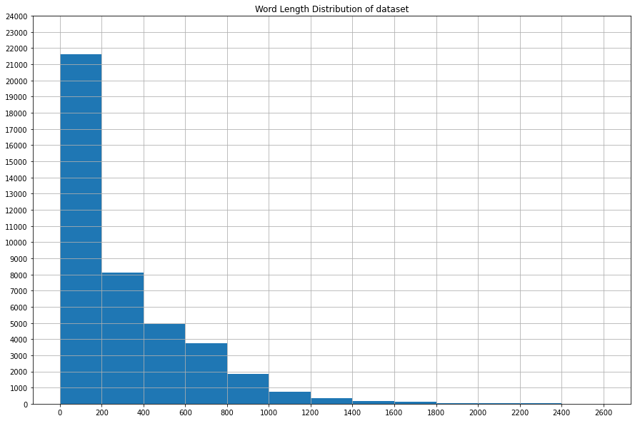
3. Text Preprocessing
Preprocess the text in order to be suitable for inputting into the model (defined later)
mean_seq_length = preprocessed_df.Movie_Summary.str.split().str.len().mean()
median_seq_length = preprocessed_df.Movie_Summary.str.split().str.len().median()
dist = list(preprocessed_df.Movie_Summary.str.split().str.len())
plt.figure(figsize = (15,10));
plt.hist(dist, bins = np.arange(0, 2700, 200));
plt.xticks(np.arange(0, 2700, 200))
plt.yticks(np.arange(0, 25000, 1000))
plt.grid(axis = 'both')
plt.title('Word Length Distribution of dataset');
train_data, val_data, train_labels, val_labels = train_test_split(data,
                                                                  labels,
                                                                  random_state = 123,
                                                                  test_size = 0.2)
train_data = np.squeeze(train_data)
val_data = np.squeeze(val_data)
train_data = train_data.astype('str')
val_data = val_data.astype('str')
# max length of the sequences
MAX_LEN = 256

# tokenizer to be used to tokenize the strings
tokenizer = BertTokenizerFast.from_pretrained('bert-base-uncased', do_lower_case = True)

def tokenize_data(max_len, data, tokenizer):
  '''
  Tokenize data and return list of tokens (input_ids, attention_mask)
  Args:
  1) max_len : maximum length of sequences
  2) data : data to be tokenized
  3) tokenizer : tokenizer to be used
  Returns:
  1) input ids
  2) attention mask
  '''
  tokenized_data =  tokenizer.batch_encode_plus(data,max_length=max_len,
                                                add_special_tokens= True,
                                                padding='max_length',
                                                truncation=True,
                                                return_tensors = 'tf',
                                                return_attention_mask = True,
                                                return_token_type_ids = False)

  tokenized_data = [tokenized_data['input_ids'], tokenized_data['attention_mask']]

  return tokenized_data
# tokenized train, val data
X_train = tokenize_data(MAX_LEN, train_data.tolist(), tokenizer)
X_val = tokenize_data(MAX_LEN, val_data.tolist(), tokenizer)
BATCH_SIZE = 16

def batch_data(data, labels,batch_size, buffer_size):
  '''
  Create and return TF dataset
  Args :
  1) data : list of tokens
  2) labels : list/array of OHE labels
  3) batch_size : size of a batch
  4) buffer_size : buffer_size for shuffling
  Returns:
  1) Tensor data that is shuffled, batched and prefetched
  '''
  dataset = tf.data.Dataset.from_tensor_slices(({'input_ids' : data[0], 'attention_mask':data[1]}, labels))
  dataset = dataset.shuffle(buffer_size).batch(batch_size).prefetch(tf.data.experimental.AUTOTUNE)
  return dataset
train_dataset = batch_data(X_train, train_labels, batch_size = BATCH_SIZE, buffer_size = 50000)
validation_dataset = batch_data(X_val, val_labels, batch_size = BATCH_SIZE, buffer_size = 50000)
4. The Model
Define the model template to be used in the training
def create_model(max_length = 256):
  """
  Creates the model using Tensorflow Functional APIs
  Args:
  1) Maximum length of sequences
  Returns:
  1) Model template to be trained
  """
  bert_model = TFBertModel.from_pretrained('bert-base-uncased')
  input_ids = tf.keras.layers.Input(shape = (max_length, ), dtype = tf.int32, name = 'input_ids')
  attention_mask = tf.keras.layers.Input(shape = (max_length, ), dtype = tf.int32, name = 'attention_mask')
  x = bert_model.bert(input_ids, attention_mask)
  x = x.pooler_output
  x = tf.keras.layers.Dropout(0.2, name = 'dropout_layer_1')(x)
  x = tf.keras.layers.Dense(256, activation = 'relu', name = 'hidden_dense_layer')(x)
  x = tf.keras.layers.Dropout(0.2, name = 'dropout_layer_2')(x)
  x = tf.keras.layers.Dense(33, name = 'dense_layer_output')(x)
  out = tf.keras.layers.Activation('sigmoid', name = 'activation_layer_output')(x)
  model = tf.keras.Model(inputs = [input_ids, attention_mask], outputs = out)
  model.compile(optimizer = tf.keras.optimizers.Adam(learning_rate=3e-5),
                loss = tf.keras.losses.BinaryCrossentropy(),
                metrics = tf.metrics.BinaryAccuracy())
  return model
model = create_model()
5. Training
Train the model on data
reduce_lr = tf.keras.callbacks.ReduceLROnPlateau(monitor = 'val_loss', factor = 0.1, patience = 1, min_lr = 1e-8)
history = model.fit(train_dataset,
                    validation_data = validation_dataset,
                    epochs = 3,
                    callbacks = [reduce_lr])
6. Checking on a stray example
Check how the model performs on a random example in the validation dataset
model.save_weights(os.path.join(PATH, 'Checkpoint/Model_Checkpoint'))
new_model.load_weights(os.path.join(PATH, 'Checkpoint/Model_Checkpoint'))
predictions = new_model.predict(validation_dataset.take(1))[0]
labels = preprocessed_df.iloc[:, 3:].columns
for i in range(len(labels)):
  if predictions[i] > 0.5:
    print(f'{labels[i]}:{predictions[i]*100}%')
7. Checking on User Input
Section to check model output on user output
MODEL_DIR = <YOUR_MODEL_DIR>
version = 1
export_path = os.path.join(MODEL_DIR, str(version))
tf.keras.models.save_model(model,
                           export_path,
                           overwrite = True,
                           include_optimizer=True,
                           save_format = 'tf',
                           signatures = None,
                           options = None)
saved_model = tf.keras.models.load_model(export_path)
data = [data]
tokenized_data = tokenize_data(MAX_LEN, data, tokenizer)
predictions = saved_model.predict({'input_ids':tokenized_data[0], 'attention_mask': tokenized_data[1]})
predictions = np.squeeze(np.asarray(predictions))
labels = preprocessed_df.iloc[:, 3:].columns
maxm = max(predictions)
for i in range(len(labels)):
  if maxm/predictions[i] <= 3:
    print(f'{labels[i]}:{predictions[i]*100:.2f}%')
action:81.47%
adventure:87.00%
animation:41.06%
fantasy:39.80%
Continue onto the next part for model deployment