We Are The World

You are not a drop in the ocean. You are the entire ocean in a drop

Rumi

Quick history lesson: When did the very concept of a nation state and all its trappings come to be? That would be the Peace of Westphalia in 1648. This landmark event formalized political boundaries, the notion of sovereignty and non-interference in state affairs and trade and commerce regulations. Before that boundaries were more fluid but of course more wars. So, while the early system favored for the plebeians, the new system ensured the elites could keep their spoils. Maybe if we took greed out, we are one? Lets explore this topic in today's blog.

We'll skim over the hierarchical agglomerative clustering model - an unsupervised learning model and use it to progressively group countries on a few key indicators. We should be able to observe some really interesting patterns emerge and draw some insights.

Hierarchical Agglomerative Clustering

Hierarchical Agglomerative Clustering (HAC) builds a "hierarchy of clusters". It creates a cluster tree or dendrogram that builds up by progressively merging smaller clusters into larger ones.

We use a "distance" metric to merge two clusters. To assign a distance between two clusters, we often use one of the following heuristics:

• Single Linkage: Distance between the closed members
• Complete Linkage: Distance between the farthest members
• Average Linkage: Average distance between the 2 clusters

When do we stop? Thats the best part - the algorithm doesn't "require" the specification of a stopping criterion. We can specify a stopping criterion such as number of clusters, height, distance threshold, etc but completely optional. However, this is also a double-edged sword (surprises!) because its computationally expensive for large datasets.

The Data

Data will last longer than the systems themselves

Tim Berners-Lee

The dataset we'll be using is pretty straightforward. It enumerates the countries in the world and their population, migration, GDP (per capita), literacy, number of phones (this came out of nowhere!) and infant mortality.

Do we need some preprocessing? Certainly. First drop the "Country" column. Next, we can see that the numerous metrics have vastly different orders of magnitude. Here, what we'll simply do is normalize each type of feature i.e. centre each feature around its mean dividing it by its standard deviation.

The Model

Complex data into simple decisions. That is the essence of machine learning.

We've prepared our data suitably. Now we need to implement the core of our model. In this blog, we'll be using complete linkage as our distance metric but we can minimally modify the code for single and average linkage as well. To prevent repeated computation of the distance metric between the tuples in the dataset, we'll first precompute and store the pairwise distances in a matrix.

def precompute_pairwise_distances(featureMatrix):
    """
    Calculate pairwise distances for all feature vectors in the matrix
    Arguments:
        featureMatrix: numpy array representing the feature matrix
    Returns:
        distances: numpy array with the pairwise distances between any two feature vectors
    """
    distances = np.zeros(shape=(featureMatrix.shape[0], featureMatrix.shape[0]))
    for i in range(featureMatrix.shape[0]-1):
        for j in range(i+1, featureMatrix.shape[0]):
            dist = np.linalg.norm(featureMatrix[i, :]-featureMatrix[j, :])
            distances[i][j] = dist
            distances[j][i] = dist
    
    return distances

The core HAC algorithm is now very simple to implement. We'll describe the steps before providing the code for these steps

• Create the feature matrix for the dataset
• Precompute and keep the pairwise distances in a matrix pwDistances
• Initialise each tuple (n tuples total) as its own cluster - groups
• We need to keep track of the merge details at every level. We do this with Z which is initialized to the correct size (n-1, 4) and filled with zeros
• Now merge clusters n-1 times to fill Z
  • Find the clusters with minimum value for complete linkage distance.
  • Use the cluster indices and values for minimum distance and the length of the new merged points to fill Z at the correct level
  • Now remove them from groups
  • Add the merged cluster to groups

QED! The code fragments for this bit are given below. Can we optimize this? (hint: use itertools to make it faster)

Plotting

The best lies are seasoned with a bit of truth

George R.R. Martin

The resulting Z can be plotted using `scipy`'s hierarchy module. We can pass the Z we obtained and the labels to the `dendrogram` and we'll have our clustered groups. Why the perhaps unnecessary quote though? It is because we're going to see the graph and try to reason why a certain grouping might have happened. In simple terms some kind of validation bias.

hierarchy.dendrogram(Z, labels=names, leaf_rotation=90, ax=ax)

Results and Insights

However beautiful the strategy, you should occasionally look at the results.

Winston Churchill

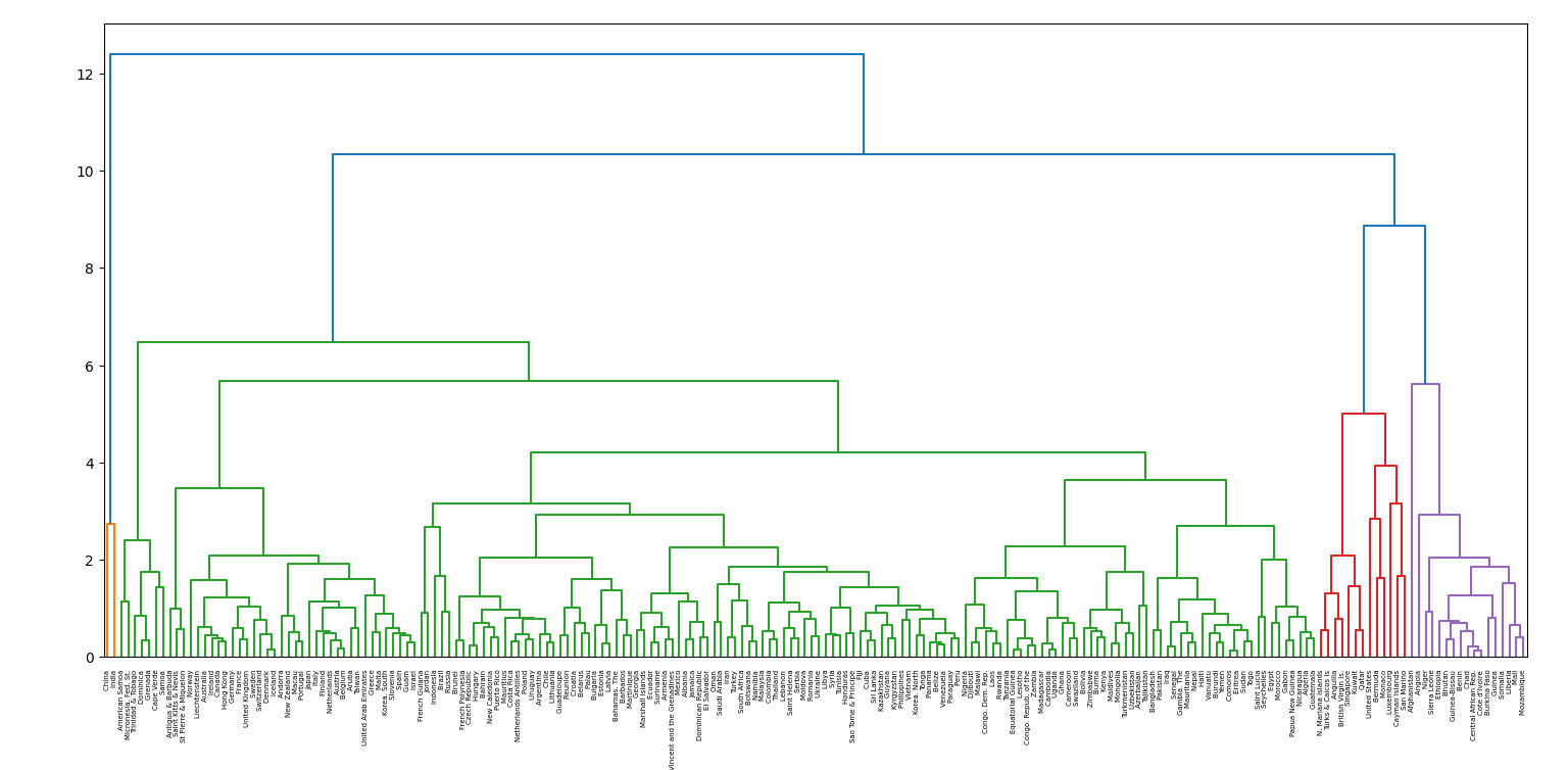
Great! Although there's too much to unpack here, we can clearly see countries with similar populations and economies being grouped together. India and China seem to stand out, merging at the end with the rest of the world. European, African and South American countries clustering together before merging with other groups. Company you keep certainly matters!

Conclusion

The strong do what they can
The weak suffer what they must
Thucydides

And thus we have demonstrated hierarchical agglomerative clustering on countries data. See you again in a new blog!